Purpose
Analysis of satellite images is a foundational technique for generating intelligence through Earth Observation (EO) and has applications in defence, agriculture, climate, natural disasters and urban management. This work takes a case study-driven approach to build data pipelines in Kubox. We map urban growth hotspots in 1,809 Australian localities using satellite images covering 30,000 km².
Outcome
By using open-source distributed computing frameworks like Dask and Dagster, we demonstrate a scalable and efficient approach to geospatial analysis. Our implementation processed 30,000 km² of Australian urban areas and their surroundings, in 90 minutes at a total compute cost of 15 AUD. This highlights how Kubox helps developers quickly test ideas, spin up the right-sized clusters exactly when needed, and use top data and AI tools to convert jupyter notebooks into repeatable and robust data pipelines.
Introduction
Tracking urban expansion is complex, especially in vast countries like Australia. The computational demands and specialist geospatial algorithms can be overwhelming. Thankfully, there are open-source software ecosystems like Open Data Cube for managing and processing gridded Earth observation data. Furthermore Geoscience Australia provides Digital Earth Australia (DEA), a fantastic free and open-source satellite imagery archive.
But here’s where it gets tricky — scaling data pipeliness to process across an entire country like Australia requires setting up complex compute infrastructure, distributed parallel execution and the capability for rapid experimentation to optimise for both efficiency and cost.
In this example, we use Kubox to provision a cluster in AWS cloud and leverage open source tools like Dask and Dagster to process satellite images.
What are urban growth hotspots?
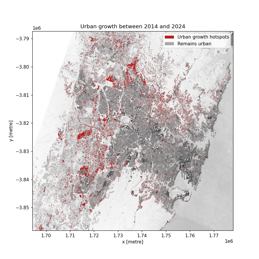
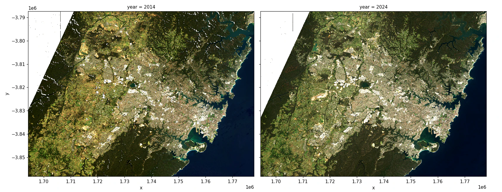
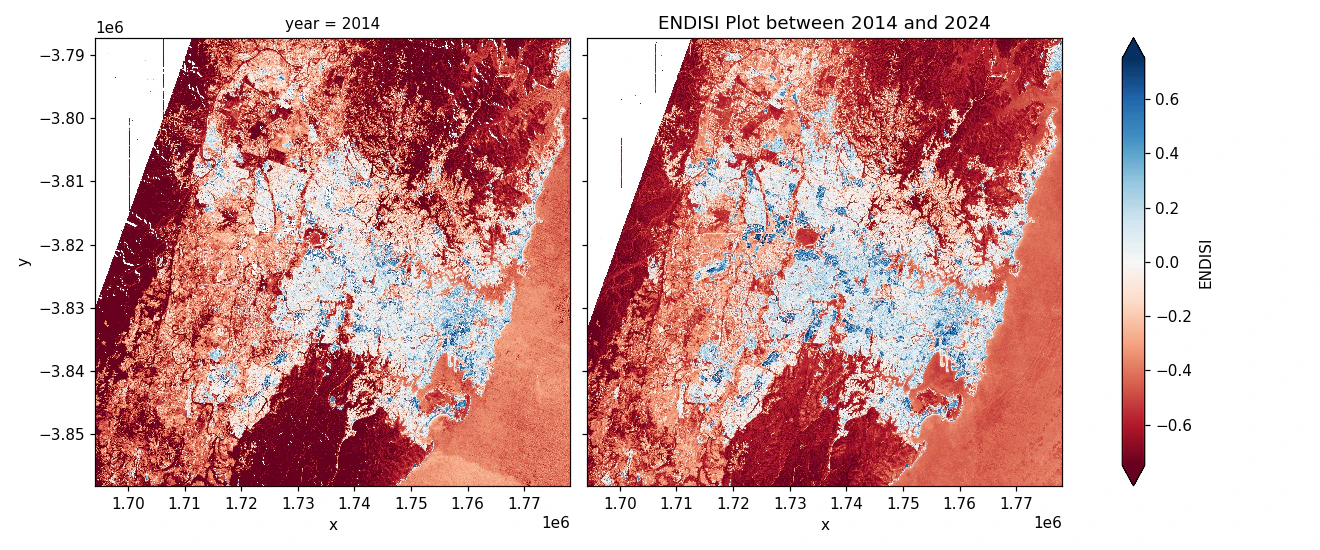
Urban growth hotspots represent the areas of urban expansion between two periods, visually highlighted on a map to show growth locations. For example, below image shows urban hotspots for Sydney comparing satellite images of 2014 and 2024.
Credits
Firstly, credit where it’s due. The original work for detecting change in urban extent has been done by Geoscience Australia. We’ve made some improvisations and necessary changes to the original code. So, while we owe a nod to DEA, our unique approach took it a step further to process at scale and speed.
Krause, C., Dunn, B., Bishop-Taylor, R., Adams, C., Burton, C., Alger,
M., Chua, S., Phillips, C., Newey, V., Kouzoubov, K., Leith, A.,
Ayers, D., Hicks, A., DEA Notebooks contributors 2021. Digital Earth
Australia notebooks and tools repository.
Geoscience Australia, Canberra. https://doi.org/10.26186/145234
Workload Characteristics
- Data Skew: 21 major urban cities make up 45% of the total area, requiring 4x more memory than smaller regions.
- DAG Pipeline: The workload requires combination of parallel and sequential execution, highlighting the need for a Directed Acyclic Graph (DAG) to effectively manage dependencies and execution order.
- Mixed I/O: The pipeline incorporates a mix of HTTP and S3 calls for loading satellite images. This causes waits and blocking if not handled separately.
- Compute Intensive Tasks: Geomedian calculation requires multiple passes over each pixel, while plots for areas greater than 2000 km² cause memory leaks for dask workers.
Solution
Data Infrastructure
With Kubox, you can quickly spin up right-sized Kubernetes clusters in your own cloud within minutes. The process begins with exploratory analysis in Jupyter notebook connected to Dask clusters for rapid prototyping. As algorithms and configurations stabilise, structured data pipelines are developed using Dagster, tested locally, and packaged as containers through CI pipelines. These containerised workflows are deployed on a new Kubox cluster, ensuring seamless execution across Dask and Dagster pods. This iterative approach enables efficient transformation of ideas into robust, repeatable production data pipelines.

Cluster Sizing and Utilisation
21 Major Urban Areas (processed in 30 minutes)
- Dask Workers: 22 instances (2 vCPUs, 8 GiB RAM each)
- Dagster Runs: 7 parallel runs (2 vCPUs, 16 GiB RAM each)
Remaining 1,788 Areas (processed in 60 minutes)
- Dask Workers: 44 instances (2 vCPUs, 8 GiB RAM each)
- Dagster Runs: 22 parallel runs (2 vCPUs, 4 GiB RAM each)
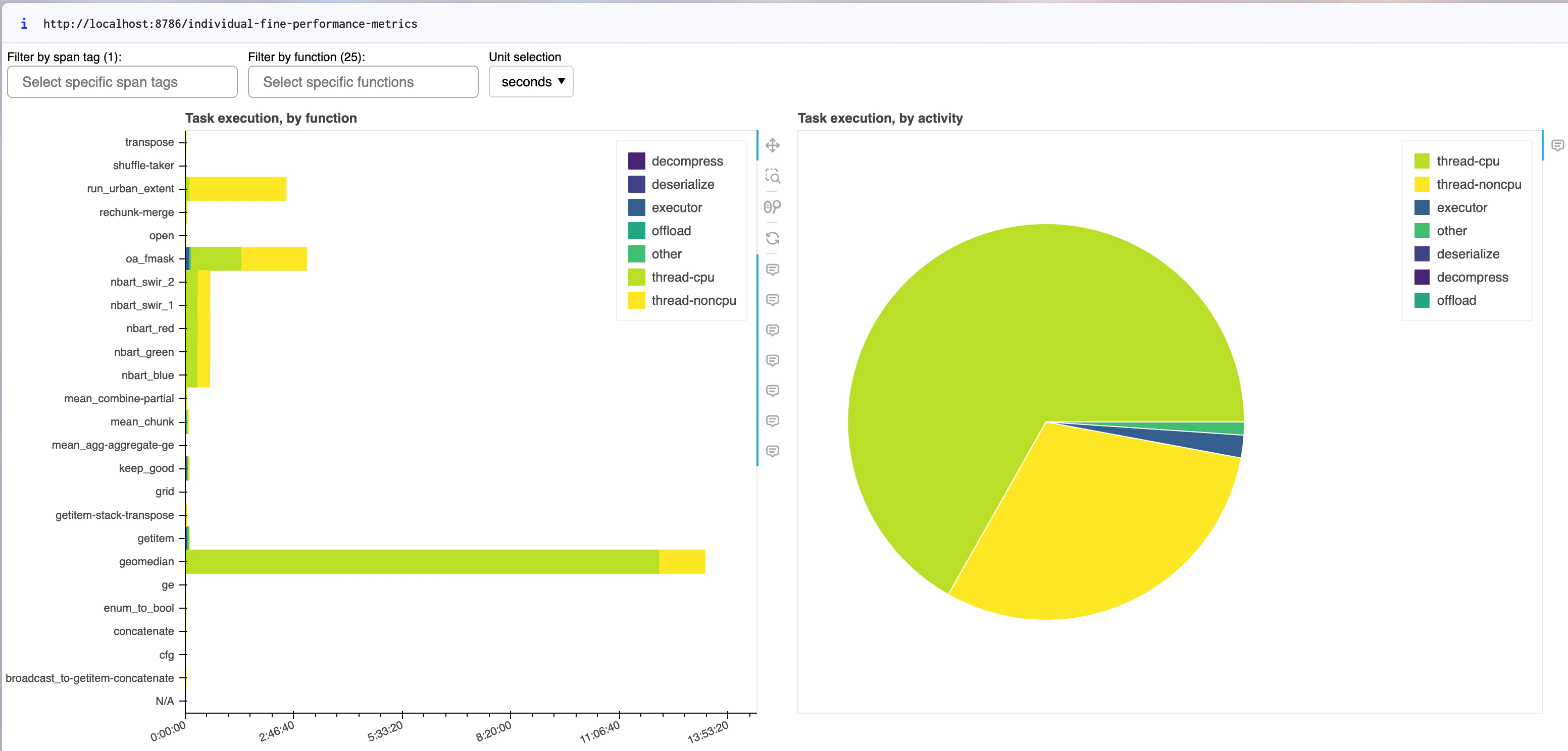
The performance metrics below were collected while running the urban extent analysis for 21 Major Urban areas. The charts display function runtime (left) and activity distribution (right). The geomedian calculation dominates execution time, consuming a large portion of CPU (thread-cpu, green) and non-CPU (thread-noncpu, yellow) resources, highlighting its computational intensity. Other tasks, such as file opening and rechunking, contribute but on a smaller scale. The pie chart confirms that most execution time is CPU-bound, with minimal overhead from executor, deserialization, or decompression, indicating efficient CPU utilisation with minimal idle time in the Dask cluster.
Costs
The estimated hourly cost of the below Kubox cluster is 9 AUD, inclusive of services such as the Load Balancer and EBS Volumes. With a total runtime of 110 minutes, accounting for cluster startup, container loading, and teardown, the overall cost is approximately 15 AUD.
| Instance Type | Hourly Rate (AUD) | vCPUs | Memory (GiB) | Quantity | Services |
|---|
| t3.2xlarge | $0.15 | 8 | 32 | 1 | Control Plane |
| t3.xlarge | $0.08 | 4 | 16 | 1 | Worker Node |
| m5.4xlarge | $0.38 | 16 | 64 | 1 | Dask and Dagster management services |
| m5.12xlarge | $2.50 | 48 | 192 | 3 | Dask Workers and Dagster Runners |
| c5.2xlarge | $0.17 | 8 | 16 | 1 | PostgreSQL |
Data Pipeline
- Input Satellite Images: We begin with official digital boundaries of urban areas, stored as a Shapefile in AWS S3. These boundaries help us identify and retrieve a list of
GeoTIFF satellite images and metadata for a specific area using the SpatioTemporal Asset Catalog (STAC) standard, accessed via a REST API provided by Geoscience Australia. For more information see STAC user guide.

- Pre-processing: This step processes multiple satellite images of a location taken at different times, removing unwanted elements like clouds and shadows to create a clear and accurate picture. We apply this process to all images captured for that location in 2014 and 2024, resulting in two final images of the location, one for each year.
- Calculate urban extent: We calculate the Enhanced Normalized Difference Impervious Surfaces Index (ENDISI) for each pixel in both year images to define urban areas. Pixels above a set threshold are labeled “Urban”, while those below are excluded. By subtracting the baseline year’s ENDISI from the analysis year, we highlight urban growth hotspots.
- Visualisation: All plots are generated using Matplotlib in headless mode and can be optionally stored in an S3 bucket. Hotspot polygons, statistics, and metadata are saved in a
GeoJSON file, with a final aggregated version prepared for map-based visualisation.
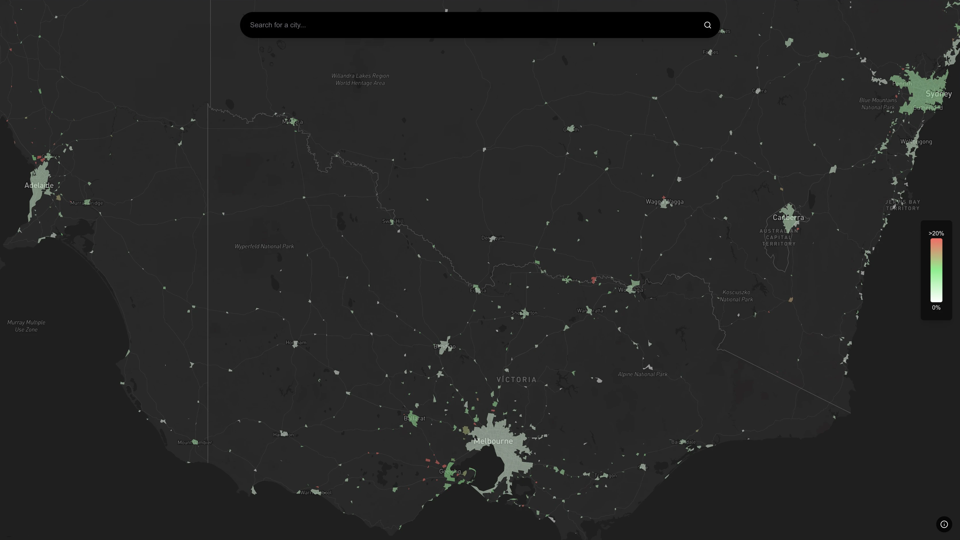
Explore the interactive map of all urban hotspots at https://urban.app.kubox.cloud
Geomedian is used in satellite image processing to help create an accurate and reliable representation of the Earth’s surface by removing unwanted variations caused by objects like clouds, shadows, etc.
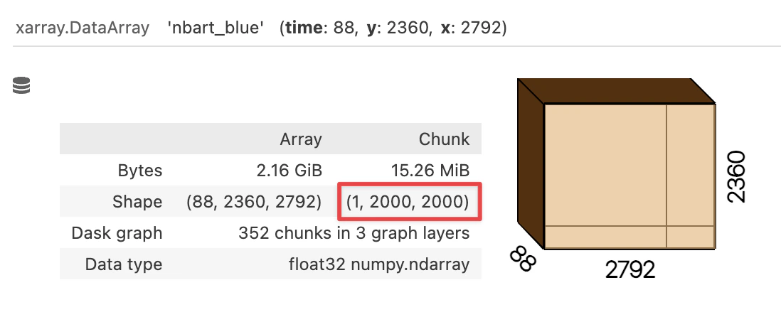
For efficient Geomedian calculation, ensure all values of a single pixel are stored in one chunk.
(1, 2000, 2000) is highly inefficient for calculating the geomedian.
 We dynamically re-chunk the dataset to
 (max_time, 200, 200), ensuring all time values for a pixel are stored in a single chunk.
ds = odc.stac.load(
    items,
    bbox=bbox,
    crs="EPSG:3577",
    bands=[
        "nbart_swir_1",
        "nbart_swir_2",
        "nbart_blue",
        "nbart_green",
        "nbart_red",
        "oa_fmask",
    ],
    resolution=30,
    groupby="solar_day",
    chunks={"time": 1, "x": 2000, "y": 2000},
    resampling={"oa_fmask": "nearest", "*": "bilinear"},
)
max_time = ds.sizes["time"]
ds = ds.chunk({"time": max_time, "x": 200, "y": 200})
ds.nbart_blue
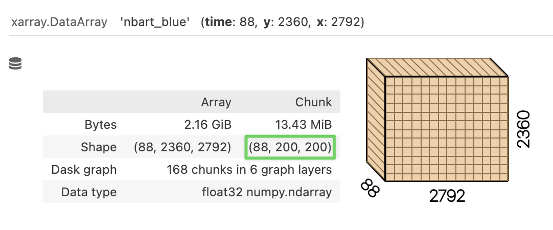
Re-chunking the xarray from (1, 2000, 2000) to (max_time, 200, 200) improves geomedian computation performance by 10x for large cities.
Background
Satellite Images Dataset
Landsat 8 is part of a suite of Digital Earth Australia (DEA)’s Surface Reflectance datasets that represent the vast archive of images captured by the US Geological Survey (USGS) Landsat and European Space Agency (ESA) Sentinel-2 satellite programs, validated, calibrated, and adjusted for Australian conditions. The resolution is a 30 m grid and radiance data collected can be affected by atmospheric conditions, sun position, sensor view angle, surface slope and surface aspect.
The Australian Bureau of Statistics (ABS) provides classification of Australia into a hierarchy of statistical areas. Statistical Areas Level 1 (SA1s) have a population of between 200 to 800 people and are designed to maximise the geographic detail available for Census of Population and Housing data while maintaining confidentiality. Urban Centres and Localities (UCLs) are aggregations of SA1s which meet population density criteria or contain other urban infrastructure. Section of State (SOS) groups the UCLs into classes of urban areas based on population size. They are:
- Major Urban — urban centres with a population of 100,000 or more.
- Other Urban — all other urban centres with a population less than or equal to 99,999.
- Bounded Locality — localities with a population up to 1,000
- Rural Balance — represents the Remainder of State/Territory
We use Urban Centres and Localities - 2021 - Shapefile, provided as part of the Australian Statistical Geography Standard (ASGS) digital boundaries. It has the below.
| Section of State Type | Area km² | Number |
|---|
| Bounded Locality | 6,169 | 1,080 |
| Major Urban | 13,463 | 21 |
| Other Urban | 9,632 | 708 |
| Rural Balance | 7,658,828 | 9 |
Insights
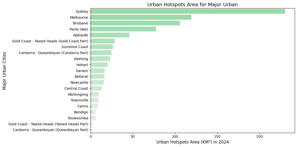
These charts show urban growth hotspots (total km²) while comparing urban extent from 2014 to 2024.
All Major Urban Areas
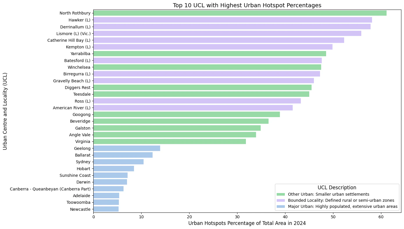
Top 10 percentage hotspots
This graph visualises the top 10 urban hotspots as a percentage of their total area for each Urban Centre and Locality (UCL) type. Smaller Bounded Localities and Other Urban areas exhibit the highest hotspot percentages, whereas Major Urban centres like Geelong, Ballarat, and Sydney show relatively lower percentages.
 This Jupyter Notebook provides some more analysis.
Source Code
Visit our Github repository at https://github.com/kubox-ai/urban-extent if you prefer to explore a small area of interest with Jupyter Notebook, start here.